In response to several misconceptions or assumptions arising from media coverage of the recent publication: “Western scrub-jay funerals: cacophonous aggregations in response to dead

conspecifics” 

–When western scrub-jays see a dead jay they alarm call and attract other jays which then may join in calling. This loud gathering or “cacophonous aggregation” lasts a few seconds to tens of minutes then the birds disperse.

–Jays did not stop eating entirely over the course of 24-48 hours. I trained them to expect peanuts in a feeder every morning and then one day they got a surprise in the form of a wooden object, a dead jay, a stuffed jay, or a stuffed owl on the ground about 1 meter from the feeder. After the dead jay and stuffed owl they reduced or stopped taking peanuts from the feeder. They had been hiding (or caching) peanuts nearby this entire time so they simply turned to those peanuts if they wanted peanuts or ate other things. 

–No jays were killed for this study. I had permits to collect (or salvage) dead birds and I made great use of these permits by amassing a respectable collection of birds killed by predators as well as cars. I had a great network of people that would call or email me if they saw a dead bird. Yes, many of the birds were very smelly and I still prepared them as dried skins for the love of the question!

–At no point do I or the other authors make statements regarding the occurrence or absence of emotions or cognitive depth in these birds in this context. The work does not address this question and realistically, there are no great methods to address such a question at this time. If there were, I would have grabbed that question by the horns…er, beak? At this time I remain agnostic about these issues but evolutionarily speaking there is probably some sort of continuity as the emotional response could conceivably act as a mechanism to facilitate outcomes that further an organism’s fitness– social and/or pair bonding is probably the most obvious.  

 

Hi all, I have recently published my first 1st-author paper after years of hard work on my PhD thesis at the University of California Davis with Gail Patricelli and Richard McElreath. 

“Western scrub-jay funerals: cacophonous aggregations in response to dead
conspecifics”

I’m very excited about the attention the research is getting. Animal behavior in general is fascinating and I’m thrilled that so many are finding how scrub jays respond to their dead as interesting as I do. Unfortunately, given the current inaccessibility to published research by the public at large, most are not able to evaluate the information first hand. At most, I believe there is access to the title, abstract and some figures. While those that have read the abstract agree that the use of the word “funeral” in the title is not problematic as there is no hint of anthropomorphic treatment of the behavior, others are at least perplexed if not potentially offended by its inclusion in the title.

I would like to clarify that indeed, the word is only included in the title and there is no further assumption regarding the emotional or cognitive state of the gathering birds. This is an agnostic stance– not a refutation or a condemnation for considering such ideas. The problem is that current methodology does not allow us to explore these questions in a satisfying and conclusive manner. Otherwise, I’d be all over that!

I decided to include the word “funeral” only as a way to link this work to previous observations and reports of many other species reacting to dead fellows. Try googling “chimp”, “elephant”, “crow”, “magpie”, “bison” and probably many other animals followed by the word “funeral”. What you come across is a lot of interesting accounts about how animals respond to their dead. I chose the term “cacophonous aggregation” to denote this behavior in western scrub-jays. In the scientific literature, “ceremonial gatherings” was used to describe magpies’ response to a fallen fellow. I thought that even this term was too suggestive so I opted for a more descriptive and agnostic term as the label.

If you google “cacophonous aggregation” at most you may come up with a link to the abstract to my paper but you would be robbed of learning about all the other interesting stories out there about how animals react to their dead. 

 

 

After months of nothing, the Science As A Verb crowd has finally made a blog post…somewhere else.

Last time we went to Curacao, we followed Losos’ advice and spent some time looking at anole dewlaps.  Matt Brandley wrote up an awesome summary of what we found over at Anole Annals.

I’m going to bash together some new original content soon, but for now I wanted to point to this excellent article over on Ewan Birney’s blog: Five Statistical Things I Wished I Had Been Taught 20 Years Ago.  Both the post and the ensuing discussion are informative.

Darryl Cunningham is the author of a series of excellent comic strips that explain and demystify important aspects of science.  His post on anti-vaccine hysteria is what originally got me hooked on his blog, but his new one on evolution is even better.  He has a great way of making complex ideas simple and succinct, and the art emphasizes the conversational tone of his writing.

I recently began using model selection methods and AIC to analyze my data as per the strong suggestion from one of my dissertation committee members. As I learn about this methodology, I am also asked to justify my interpretations to other members of my committee. Switching over definitely has been a very productive learning experience. I thought I would share some of the questions I’ve gotten and how I responded. My responses are derived from my understanding of readings and discussions with others. I publicly air my responses for several reasons. First, there may be others out there asking these same questions and perhaps this will pop up in a search and be helpful. Second, I want others that know more to correct me (constructively!) and help me gain a deeper understanding. In keeping with the first reason, having others’ comments and corrections next to my own statements will hopefully not lead too many astray should there be gross falsehoods in my statements.

What criteria allow you to conclude that X₃ has predictive value when the wAIC for model 1 is only a bit stronger than what I assume is the null model?
The criteria I used here was a difference in AIC score of 3 or more between models. The absolute AIC score is not meaningful but the differences in scores between models can be used as a rough guideline according to Burnham and Anderson in their 2002 book (Model Selection and Multimodel Inference pp 70 and pp 446). They state that “models within 1-2 of the best model have substantial support”. [Although, I have not been able to find a theoretical justification for these rough cut-offs!] Some authors have used a cut-off of 2 and others of 3. I decided to use 3 to be more inclusive of alternative models or more conservative with criteria that a model was ok to stand alone.
When differences (ΔAICc) are within 3 units then that means that those models are plausible too so in order to get an estimate of the effect of the variables included within all plausible models you can do model averaging. Model averaging weights the variables in the model by the AIC weight and adjusts the estimate accordingly. For example, in the model set below, the estimate for “X₃” is adjusted down when you look at the averaged model. However, X₃ still has a positive effect on the response variable Y while X₁ and X₂ have estimates close to zero. Notice also that there is more uncertainty around the estimate for X₃ after averaging. One of the things this suggests to me is that there are relevant X-factors that were not measured and included as potential predictive variables. I have nothing to back this up but the fact that the second-best model is the “null” suggests to me that a lot of the variation might be due to the random factor (not shown in the models below).

Comparing models with small differences in AIC score

After I compared models 1-4 and noticed they were all within 3 ΔAICc of the top model I decided to make model number 5 to see if it would rise to the top. Apparently the penalty of having three times the number of parameters trumped any combined power to predict the response variable.  All of these models also contain site as a random intercept so the variation in y seemed to be due primarily to differences in site and X₃.

What I finally decided to do in this case was to use a cut-off of 2 ΔAICc, not average the models and interpret the results based on the relative weights of the models. …  this suggests that X₃ may have some effect but results are inconclusive.

This is again an example of the general question on what you can say about your results when your wAIC value for your ‘best model’ is not 0.95, but only 0.88 or 0.63, or 0.44.
The weights are calculated using the differences in the AIC score but the weight is also affected by the number of models you have in a set. Since the weights must add to 1, as you add more models some of that weight is “claimed”. So if you have a lot of models in your set the top model can have an AIC weight that is far below say 0.95 but it’s the combined evidence of difference in score, AIC weight and CI is used to determine if competing models are also plausible.
The weights are also useful in model averaging for adjusting the relative contribution of model parameters. Actually, Burnham and Anderson have stressed that model averaging should be done with all hypothesized reasonable models instead of using a cutoff in the score differences. If model averaging is done then parameters that have little impact will have a low estimate (relative to the other parameters in the averaged model if estimates are standardized) and one can see this at a glance. However, standardizing the estimates for different variables may be difficult to impossible. I think their main point is that the primary benefit of model averaging is to develop a more predictive model.

The best model is not necessarily a good model – its just the best out of the ones that you elected to include.
Absolutely correct. However, if you populate the model set with models that can’t predict the response variable then the “null model” (intercept-only model) will be the “best” model. If the null model is the best of the set, this doesn’t necessarily mean “no difference” it means that IF there is a difference it is not explained by the variables in your alternative hypotheses. Additionally, you can use confidence intervals or SE for model estimates in your best models to see how confident you can be that the variables included can explain the variation in the response variable.

How did you choose which models to include?
Personally, I chose to include models that I reasonably thought might be meaningful AND where the independent variable was something I had manipulated in the experiment. Choosing your models is really not different from developing alternative models to test in a study.

For standard stats, if you test 20 hypotheses, you need to adjust your p-value for multiple tests.  Is there an analog with wAICs where when you have so many ‘sets’ that you need to account for the fact that some wAIC of 0.8 or whatever really aren’t meaningful?
When I did the experiment the plan was that I was going to use null-hypothesis testing and that meant I would have to do a long series of “does such-and-such have an effect? yes/no“.
In that case it might make sense to correct for multiple tests as the probability of getting some “yes” answers can increase with the number of times asked. However, (I think) it is more important to use a correction when asking the question multiple times using different explanatory variables (X₁, X₂…) for the same response variable (Y). In my case, I was asking whether stimulus alone affected the outcome and used no other explanatory variables in an attempt to keep “hunting” for a significant result. Therefore, originally I was not incorporating a multiple-test correction in my stats methods.

By using model selection on the surface it does seem that I am asking many times whether variable X₁, X₂, X₃… can predict variable Y. The big difference is that it is not a “game” of probability. If X₁ has any power to explain variation in Y then you get an estimate of the magnitude of that effect with some measure of precision. Rather than just get a yes/no answer that “X₁ has an affect” you get a measure of the magnitude of the effect which is not subject to probability.

You do alter your “chances” of getting models with high AIC weights by using fewer models in a set since each additional model can “claim” some of the total weight of 1 and dilute the pool. However, the weight is not the only selection criteria and there is also not a cut-off so that models below a certain weight are obviously meaningless. That the number of models can affect the spread of weight doesn’t change the chances that your pet alternative hypothesis ends up being the “best” model. If none of the alternative models have predictive power then it’s the “null model” that ends up with the greatest support. This result is not a matter of probability but a matter of developing reasonable, meaningful models.

Personal take:
One of the benefits I’ve seen from using model selection rather than null-hypothesis testing is that it has allowed me to understand what I’m observing in greater detail in a relatively painless way. I know there are more complicated stats (beyond t-tests and non-parametric equivalents) that allow you to see these patterns but I never felt comfortable with the methods. I did not doubt their validity! I simply felt overwhelmed by the assumptions and the need for correcting for multiple tests and basically the logistics of performing a complex MANOVA or worse yet, finding a legitimate non-parametric way to ask the questions I wanted to ask. Fortunately, I had analyzed my data using simple tests and had significant p-values for many of my comparisons. This allowed me to see that model selection was also detecting these differences so the methods were “in agreement”. Model selection allowed me to explore beyond the dichotomous treatment of my data in a way that was more transparent to me. More importantly, it allowed me to get an idea about the impact of different variables rather than a yes/no answer. Again, I’m not saying it can’t be done with “p-value” methods but I have found that for me model selection is more approachable and it helps that there are reasoned arguments to prefer model selection methods over dichotomous p-values assessments. I don’t think for one second (nor have I seen others state) that a shift to model selection as a superior method invalidates experimental results analyzed and evaluated using p-values as criteria.  In my opinion, if anything, perhaps using p-values as criteria rather than model selection has resulted in more type II errors.

I know it’s kinda lazy of me to just post a link to someone else’s blog, but holy shit this rules:

http://theoatmeal.com/comics/angler

 

 

So we’ve established that it’s often difficult to get an estimate of species’ environmental tolerances experimentally.  What’s the alternative?  Well, one alternative is to look at the set of conditions under which our species occurs naturally.  When scientists go out to collect or observe organisms in the wild, they frequently provide specimens or observational data to museums or other data storage centers.  Part of the data that is often submitted is locality data – where did you see/catch the species in question?  This data used to be in the form of verbal descriptions or rough estimates of latitude and longitude from maps, but nowadays is more often provided as GPS coordinates.  It turns out that this data is very useful in estimating species environmental tolerances and preferences.

In the most general sense, here’s how niche modeling works.  First, we have a set of occurrence points for our species:

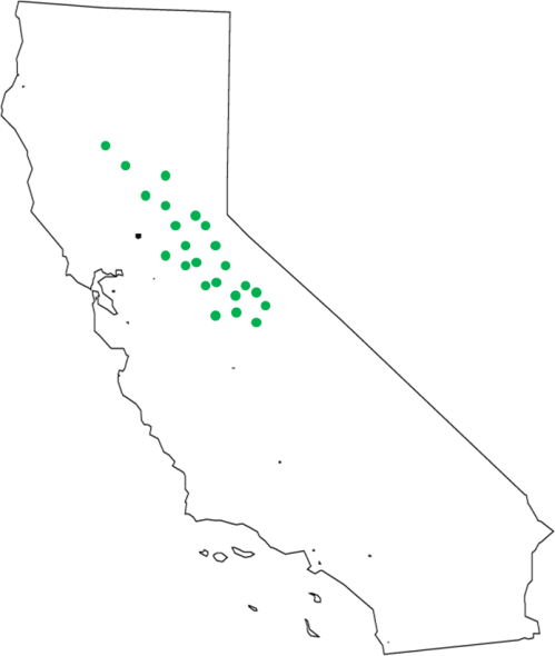
Each of these occurrences represents an observation of a set of environmental conditions under which we know our species can persist.  Unfortunately, though, this occurrence data almost never comes with direct estimates of all of the environmental factors which are potentially relevant to determining the distribution of the species.  However, we now have very fine-scale data sets containing localized estimates of a bunch of different environmental factors over the entire planet.  We can use that data in conjunction with our occurrence data to estimate the sets of conditions under which our species has been found, by extracting the environmental conditions present at each of those occurrence points.

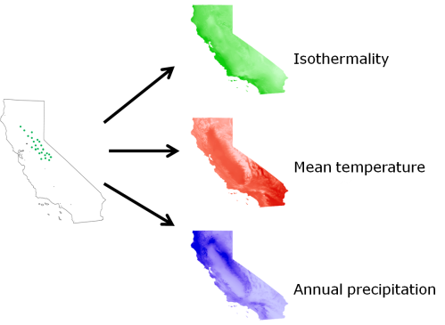
So where we once just had a bunch of latitude and longitude measurements, we now have a set of conditions that we know our species can handle, at least in the short term (if you look back at the definition of the fundamental niche you’ll see a problem here, but we’ll get to that later).  This is a valuable resource, because we can use these estimates to start building mathematical models of the environmental tolerances of our species.  There are a zillion different methods for building these models, but that’s a discussion for another time.  Suffice to say that we now have a set of points in environment space that we have extracted from our points in geographic space.  Like so:

Environmental niche modeling is simply the application of some algorithm to estimate species tolerances from this sort of data.  They range from very simple heuristics, such as “take the central 95% interval of the species distribution for each environmental variable”, which looks something like this:

To highly complex methods based on algorithms from machine learning that compare the points where the species can be found to the sets of habitats in which they have not been found:

Once we’ve got our model, we can project it back onto the geographic distribution of environmental variables to estimate the suitability of habitat across the entire geographic space.  In summary, the process looks something like this:

Where the colors on the final figure represent the estimated suitability of habitat for our species (note that in this case I just picked a model from the pile I had for California, it is not based on the points in the illustration).

This is a tremendously powerful thing, to the extent that our models can be trusted – it not only tells us something about the environmental tolerances of our species, it can tell us where we might look for populations that we haven’t seen yet.  We can also take the mathematical model of the species tolerances that we constructed in this process and project it onto environmental conditions in other geographic regions to model the ability of the species to invade other areas, or even project it onto estimated conditions in the past or future to estimate the historical or future distributions of species given various scenarios of climate change.

I have glossed over some very serious methodological and conceptual issues with niche modeling in this post, but this is intended as an introduction only.  I’ll get to the ugly bits later.  There are also some serious methodological issues that arise with transferring models to other geographic regions or time periods, but we’ll save those for another day too.  For now we’ll concentrate on the contrast between these methods and the experimental physiological methods I discussed in my last Serious Science Post (i.e., not the post about iguanas farting in the bathtub or various creatures delivering interspecific high fives).

Remember that one of the key issues with physiological niche estimates is their tractability – it is very difficult to get fine-scale estimates of the limits of species tolerances, and becomes increasingly difficult with the addition of more variables.  That’s not anywhere near as much of an issue here – all we have to do to get a new data point for our species is to see it while we have our GPS in hand.  That’s a wonderful thing, because it means that we can amass large amounts of data with minimal effort.  Since environmental variables vary over space, we can also get estimates of the response of our species to a great number of environmental variables at once with the same set of occurrence data.

So what’s the catch?  Well, it actually turns out that there are a heck of a lot of them.  I’ll probably do several posts on key methodological issues with niche models, but I’ll start just by pointing this one out: not all combinations of environmental variables occur in the real world.  Going back to our diagram from before:

We see that our species is perfectly happy in the hottest extremes of our environment space (i.e., the farthest to the right).  What if they were happy in even hotter temperatures?  We have no way of knowing whether that’s true or not, because we’ve already found them in the hottest places available to us!  Likewise, maybe they can handle higher precipitation levels in those hotter climates than they can in colder ones – it certainly looks like there might be a positive correlation between their tolerances for precipitation and temperature.  Once again, we have no way of knowing because there are no extremely hot and extremely wet regions from which we could possibly sample (or fail to sample) our species.  If we were taking an experimental approach we could simply expand the range of conditions we were testing our species under, but that doesn’t work here – as my mother always told me, we can’t afford to heat the whole outdoors.

This is a serious issue – it means that our ability to estimate the niche is limited not only by our number of occurrence points, but by the distribution of environmental variables in the study region.  This issue is serious enough that it has led some people to suggest that we not think of these methods as niche estimates at all, referring to them instead as “species distribution models”.  While I’m sympathetic to that, I still use the term “niche model” for reasons I’ll clarify in a later post.

In summary, niche modeling overcomes a lot of the difficulties that arise with physiological estimation of the niche, but brings a whole slew of other issues along with it.  TANSTAAFL, as always.

One of these days they’re going to confiscate my Ph.D., I just know it.

Vodpod videos no longer available.

Some behaviors are remarkably conservative over…, posted with vodpod

Coral reefs have the highest biodiversity of any marine ecosystem. I’ve always been fascinated by all of the critters present on reefs, and have wondered how communities are assembled, both in space and in time. We (that is, the public, as well as research scientists) immediately think about swarms of colorful fishes and complex networks of corals when we think about reefs. However, there is another level of biological complexity on coral reefs. This is the microbial communities found living on and near corals.

Acropora palmata, the elkhorn coral

Corals are unique animals in that they are intimately associated with both their constituent microbial communities and the zooxanthellae that live in the coral tissue. These three components – the coral, the zooxanthellae, and the microbes – make up the coral holobiome. With the advent of next generation sequencing it is possible to characterize the entire community of microbes living on and in association with corals. This allows testing of classic hypotheses related to community assembly. Because the microbial community is intimately associated with the host coral, inferred patterns and processes can “scale up” to the level of the host.